Optimising E-Commerce Delivery Logistics — Full Analysis

A large UK packaging ecommerce retailer was seeking to increase their profits by conducting deliveries within a set radius in house rather than using third party couriers.

I led a team of 4 analysts to determine what the optimal in house delivery strategy should be.

Step 1 - Problem Breakdown and Determining Analysis Approach

We used a fishbone diagram to disaggregate the problem question “should the client bring deliveries in house?” before settling on our analysis approach.

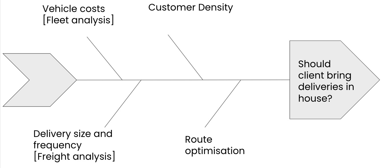
We decided on three questions to tackle the analysis:

• Profit Impact: How would bringing deliveries in-house affect profitability?
• Optimal Fleet Size: What is the ideal fleet size to efficiently manage its delivery operations?
• Optimal Delivery Freight: What delivery freight model would be best in terms of cost and operational efficiency?

We settled on 4 objectives for the analysis:

1. To create a model that will predict the profitability of a delivery route
2. Be able to predict which routes within a 50 mile radius will be profitable to undertake in house
3. Gain a better understanding of the most important factors affecting in house delivery profitability
4. Test accuracy of the model with external software

Step 2 - Data Cleaning and Wrangling

We conducted EDA to:

• Understand the data structure
• Identify trends, relationships, and anomalies

Based on the findings, we cleaned and merged the datasets. Used the Postcodes.io API in Python (with pandas and requests libraries) to generate coordinates of all orders in the customer data.

Using the Google Distance Matrix API, we calculated distances from the client base to all coordinates (n=23,178), processed in batches of 25.

Step 3 - Clustering Analysis

We used K-means clustering to analyse the relationship between:

• Customer orders and location - Customer Density
• Delivery costs and pallet space utilisation

Customer orders and location - Customer Density

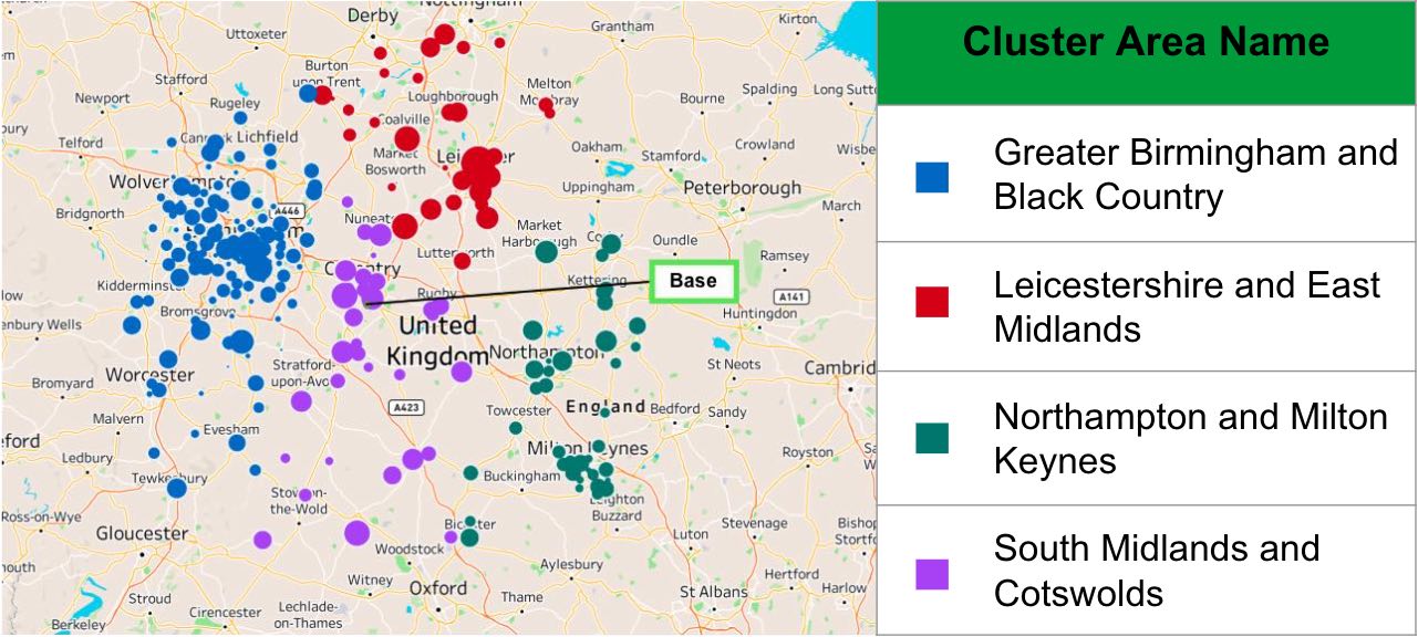
Based on the longitude and latitude we grouped the orders by area so that we could optimise delivery routes by consolidating orders within close proximity. The Elbow and Silhouette methods determined the optimal number of clusters, revealing 4 clusters.

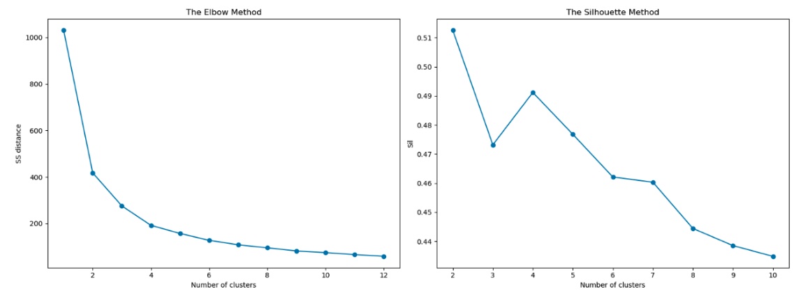
Tableau was used to visualise the data and area names were assigned.

Delivery costs and pallet space utilisation

Our key objectives were to identify orders that are disproportionately expensive relative to the space they consume and to find a group that offers a balanced representation of revenue and costs. The Elbow and Silhouette methods determined the optimal number of clusters, revealing 7 clusters.

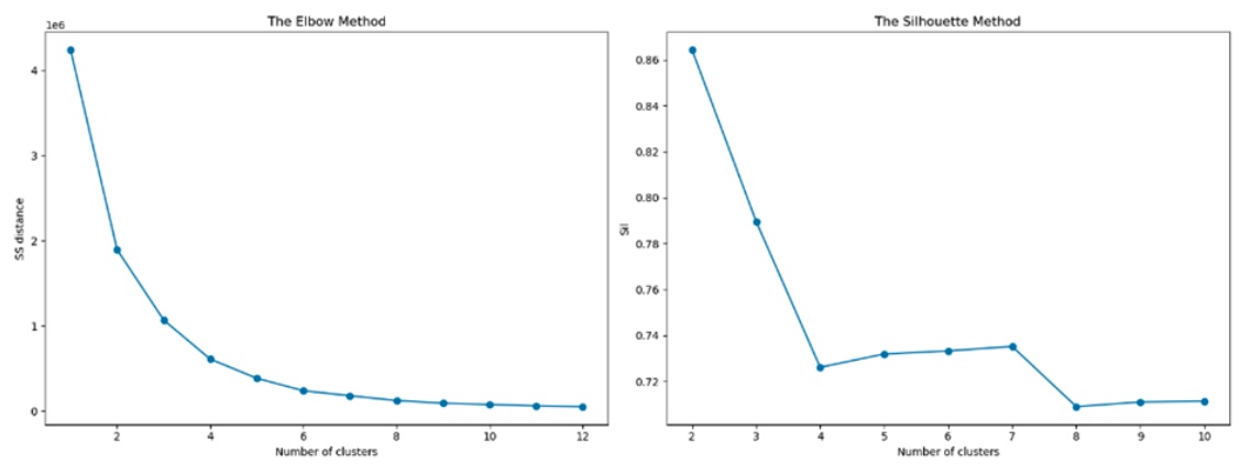
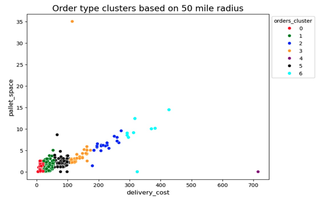
After reviewing the above, removed 2 clear outliers, resulting in 6 clusters.

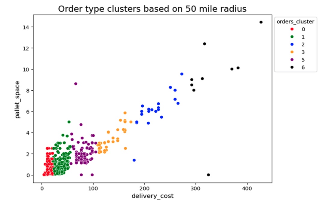
We reviewed the key metrics, and three distinct segments emerged.

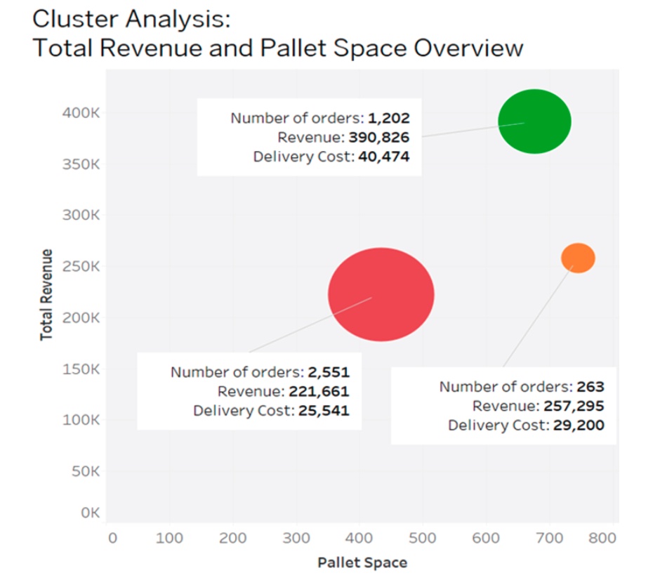
The red cluster has a high volume of orders but is characterised by low value per order and low pallet usage. These orders are resource-intensive, requiring many deliveries to achieve significant revenue, stressing daily operational limits.

The orange cluster comprises large, high-value orders that, although low in volume, offer substantial revenue but significant pallet usage. This group has the lowest cost and revenue ratio per pallet and a high value per order.

The green cluster strikes a balance with moderate order volume and pallet capacity. This group has the highest revenue and cost ratio per pallet and above-average revenue per order. This suggests that potential savings could be achieved by insourcing, thus reducing the cost per pallet while maintaining good revenue coverage.

We chose to focus our testing on the green cluster.

Step 4 - Route Optimising

We used Python and Google Directions API to optimise daily routes which involved:

• Filtering orders by type, location, and weekday (Monday to Friday)
• Setting parameters: max stops and 8 minutes per stop
• Using longitude and latitude to plan optimal routes
• Making API calls for stop-by-stop analysis
• Exporting results to CSV and Excel files

Driver Duration

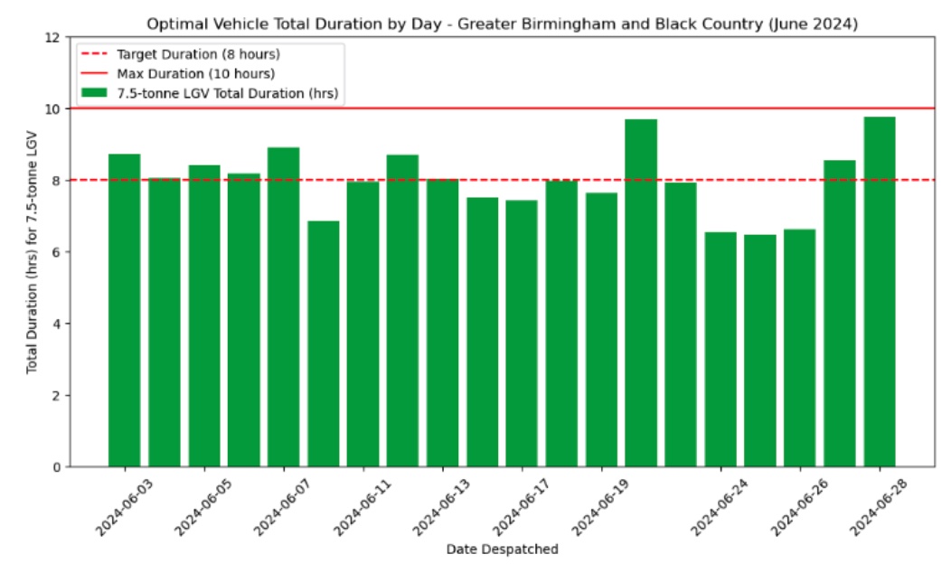
An important goal was to keep the vehicles on the road for as long as possible. The output allowed us to see the total driving duration for each route which we wanted to hit the target of 8 hours or as close to, not exceed the maximum allowed driving time per driver of 10 hours.

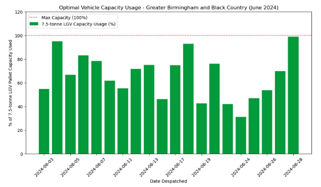
Vehicle Capacity Used

An important goal was to have the fleet as full as possible. Based on the results of the route optimisation we were able to see how the vehicle usage varies over the month of June (pallet space, cubic and payload).

Step 5 - Predicting Cost Savings

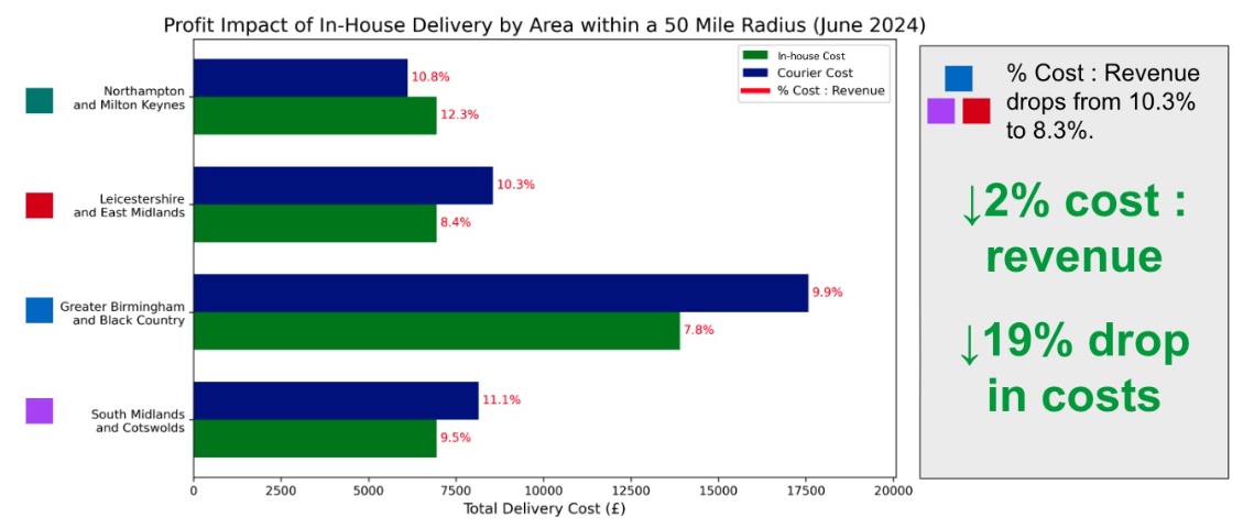
Using Python, we optimised vehicle type and fleet size for each location. The result was 4 LGVs, ensuring pallet capacity was met. This fleet size enabled cost savings based on pre-agreed vehicle cost assumptions with the client.

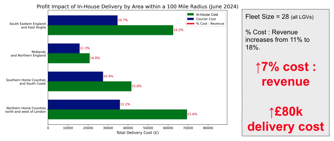
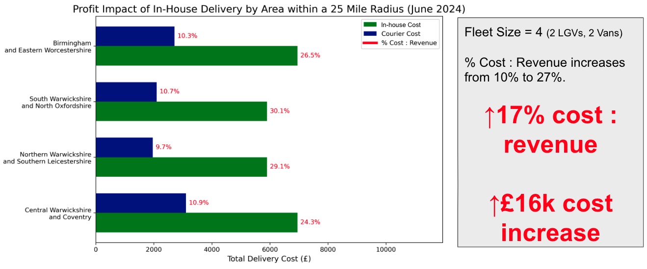
We tested the model on a 25 mile and 100 mile radius using the same methodology as the 50 mile radius. Both returned delivery cost increases for the client.

Testing the Results

Using Tableau and Excel we compared the results in terms of hours and kilometres between the Python optimiser and Routific.

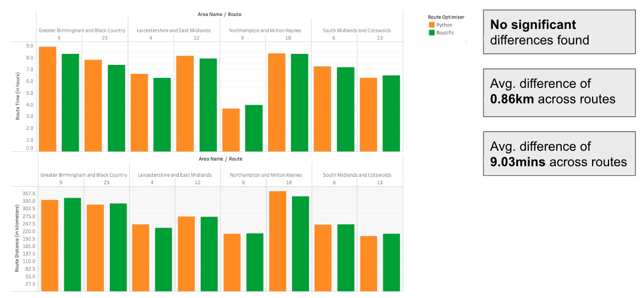
The results shown in the chart above provided confidence in the accuracy of the route optimiser built in Python.

Step 6 - Provided Insights and Recommendations

Insights:

• Clustering within a 50-mile radius of the distribution centre enabled grouping areas based on order volumes.
• The most profitable routes to manage in-house deliveries are:
  • Greater Birmingham and Black Country
  • Leicestershire and East Midlands
  • South Midlands and Cotswolds
• These routes combined could achieve a total monthly cost savings of £6.5k.
• Operating with four 7.5-ton LGV vehicles and four drivers working 8-hour shifts from Monday to Friday is sufficient to cover the proposed routes.
• Transitioning to in-house deliveries for these areas would reduce delivery costs as a percentage of revenue by 19%.
• Prioritising high-revenue orders (those offering stronger returns per pallet) will enhance profitability while maximising the utilisation of available resources.
• Deliveries for customers located between 25 and 100 miles from the warehouse, with the proposed fleet configuration, would not be cost-effective to manage in-house.

Recommendations:

• Client can achieve profitability by transitioning certain delivery routes to in-house operations. To implement this, client should acquire four 7.5-ton LGV vehicles and hire four drivers to cover the three proposed routes with a Monday-to-Friday schedule.
• The monthly operational cost is estimated at £27,800 (excluding vehicle purchase costs).
• Client should establish agreements with courier services as contingency options to mitigate operational risks, ensuring continuity in case of fleet or driver issues.